Video Swin Transformer
2021년 6월 24일 arXiv에 올라온 Video Swin Transformer를 Review하고자 합니다.
Abstract
최근 Vision분야 아키텍쳐는 일반적으로 많이 활용되는 CNN에서 Transformers구조로 바뀌고 있는 상황이고 특히 Pure Transformer Architecture의 경우 major benchmarks에서 최고의 성능을 보여주고 있습니다. Image에서 시간축이 확장된 Video models의 경우에는 Spatial, Temporal 정보를 통해 Patch를 구성해야 합니다. 본 논문에서는 Swin Transformer[1]구조를 Video에 도입하여 기존에 video recognition에서 Convolution-based backbone이 가지고 있던 inductive bias와 spatial and temporal domain에서의 speed-accuracy trade-off의 문제를 해결하면서 video recognition benchmarks(Kinetics-400, Kinetics-600, Something-Something v2)에서 SOTA를 달성하였습니다.
- Official Implementation Repo : https://github.com/SwinTransformer/Video-Swin-Transformer
1.Introduction
Transformer 아키텍쳐는 Video의 patch정보(3D)를 linear embedding을 통해 global하게 spatiotemporal relationships을 이해할 수 있는 특징이 있습니다. 또한 video recognition에서 spatiotemporal 정보의 Global self-attention을 적용하게 되면 높은 연산량과 큰 파라미터가 필요합니다. 이를 해결하기 위해 지금껏 factorization과 같은 접근을 통해 정확도는 유지하면서 연산량을 감소시킬 수 있었습니다. 하지만 본 논문에서 제안하는 Swin Transformer의 경우 spatial locality에 대한 inductive bias를 포함하면서도 hierarchical structure와 translation invariance(위치 변화에 영향이 없음)하게 구성하고 연산량을 줄이기 위한 non-overlapping windows와 shifted window mechanism을 적용하였습니다. 또한 작은 pre-training dataset(ImageNet-21K vs JFT-300M)을 통해서도 좋은 성능을 보여주고 있습니다.
2.Related Works
CNN and variants
CNN은 오랜기간 computer vision 영역에서 표준화된 backbone으로 활용되어 왔습니다. CNN의 경우 input value의 위치가 변함에 따라 feature map value도 변하는 translation equivariance한 네트워크입니다. 또한 locally connected한 성격 때문에 inductive bias가 있습니다.
Self-attention/Transformers to complement CNNs
Self-attention의 경우 long range 정보를 볼 수 있음에 따라 CNN과 함께 상호 보완적으로 Self-Attention block을 적용하여 연산량과 파라미터 수를 줄이는 Non-local neural networks가 활용되어 왔습니다.
Vision Transformers
ViT와 같이 CNN이 없는 순수 Transformer-based 아키텍쳐의 경우 inductive bias는 적은 편이지만 많은량의 data를 필요로 합니다.(e.g. JFT-300m) 반면 Swin Transformer의 경우 ImageNet만으로도 더 좋은 성능을 달성할 수 있게 되었습니다.
3.Video Swin Transformer
3.1 Overall Architecture
Video에서는 input 값이 T x H x W x 3(3D Patch)로 구성되는데 Video Swin Transformer의 경우 Figure 1과 같이 3D Patch의 사이즈를 2 x 4 x 4 x 3의 token으로 구성하여 실재 토큰의 수는 아래와 같이 나눠지고 $\frac{T}{2} \times \frac{H}{4} \times \frac{W}{4} 3 \mathrm{D}$ 로 구성된 각각의 토큰은 96 dimensional feature(channel)로 구성됩니다.
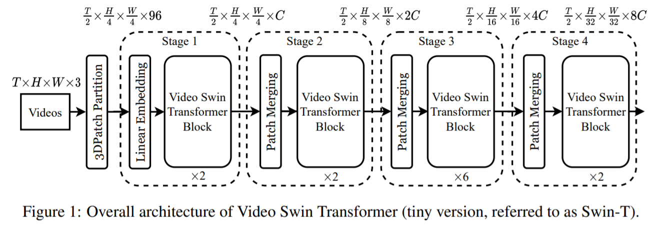
각 Stage별로 temporal dimension에서는 down sampling를 수행하지 않고 spatial dimension에 대해 2× patch merge를 통해 downsampling이 수행됩니다. Video Swin Transformer Block이전에 수행되는 Patch Merging Layer에서 2 x 2의 인근 Patch를 concatenate하여 merge한 후에 각 Patch의 channel을 2배 증가시킵니다.
- mmaction/models/backbones/swin_transformer.py
class PatchMerging(nn.Module):
    """ Patch Merging Layer

    Args:
        dim (int): Number of input channels.
        norm_layer (nn.Module, optional): Normalization layer.  Default: nn.LayerNorm
    """
    def __init__(self, dim, norm_layer=nn.LayerNorm):
        super().__init__()
        self.dim = dim
        self.reduction = nn.Linear(4 * dim, 2 * dim, bias=False)
        self.norm = norm_layer(4 * dim)

    def forward(self, x):
        """ Forward function.

        Args:
            x: Input feature, tensor size (B, D, H, W, C).
        """
        B, D, H, W, C = x.shape

        # padding
        pad_input = (H % 2 == 1) or (W % 2 == 1)
        if pad_input:
            x = F.pad(x, (0, 0, 0, W % 2, 0, H % 2))

        x0 = x[:, :, 0::2, 0::2, :]  # B D H/2 W/2 C
        x1 = x[:, :, 1::2, 0::2, :]  # B D H/2 W/2 C
        x2 = x[:, :, 0::2, 1::2, :]  # B D H/2 W/2 C
        x3 = x[:, :, 1::2, 1::2, :]  # B D H/2 W/2 C
        x = torch.cat([x0, x1, x2, x3], -1)  # B D H/2 W/2 4*C

        x = self.norm(x)
        x = self.reduction(x)

        return x
Video Swin Transformer block에서는 일반적으로 Transformer layer에서 많이 사용되는 multihead self-attention (MSA) module을 3D (shifted) window based multi-head self-attention module로 바꾸고 feed-forward network의 경우 2 Layer MLP와 GLUE로 구성되고 Layer Normalization이 적용되기 전에 residual connection이 각 모듈에 적용됩니다. 수식과 그림은 아래와 같습니다.
\[\begin{aligned}&\hat{\mathbf{z}}^{l}=3 \mathrm{DW}-\mathbf{M S A}\left(\mathrm{LN}\left(\mathbf{z}^{l-1}\right)\right)+\mathbf{z}^{l-1} \\&\mathbf{z}^{l}=\mathrm{FFN}\left(\mathbf{L N}\left(\hat{\mathbf{z}}^{l}\right)\right)+\hat{\mathbf{z}}^{l} \\&\hat{\mathbf{z}}^{l+1}=3 \mathrm{DSW}-\operatorname{MSA}\left(\mathbf{L N}\left(\mathbf{z}^{l}\right)\right)+\mathbf{z}^{l} \\&\mathbf{z}^{l+1}=\mathrm{FFN}\left(\mathrm{LN}\left(\hat{\mathbf{z}}^{l+1}\right)\right)+\hat{\mathbf{z}}^{l+1}\end{aligned}\]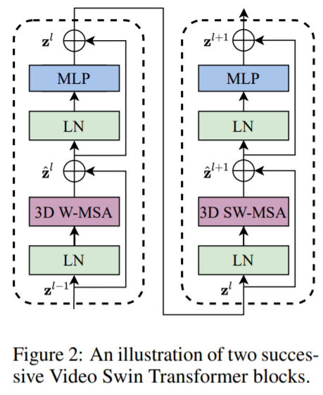
3.2 3D Shifted Window based MSA Module
Multi-head self-attention on non-overlapping 3D windows
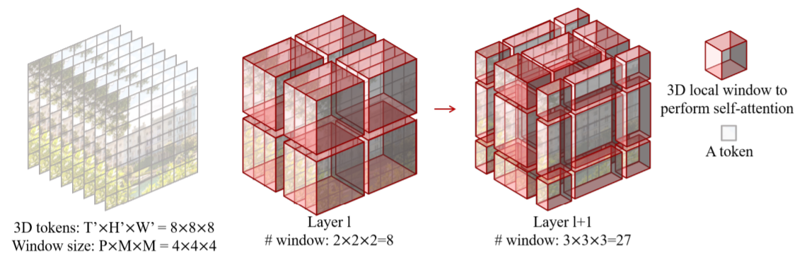
Video의 경우 시간축의 정보로 인해 Image보다 더 큰 token으로 표현을 해야합니다. 따라서 Global Self attention을 적용하기에는 매우 큰 연산량과 메모리를 필요로 하게됩니다. 이를 해결하기 위해 T’ x H’ x W’ 3D Token과 3D window size의 P x M x M로 정의하여 $\left\lceil\frac{T^{\prime}}{P}\right\rceil \times\left[\frac{H^{\prime}}{M}\right\rceil \times\left\lceil\frac{W^{\prime}}{M}\right\rceil$ non-overlapping 3D windows를 생성합니다. 예를들어 아래의 그림과 같이 input size가 8 x 8 x 8 tokens와 window size가 4 x 4 x 4인 경우 각 patch가 합쳐진 window는 2 x 2 x 2로 나누어져 각 3D token별로 multi-head self-attention이 수행됩니다.
3D Shifted Windows
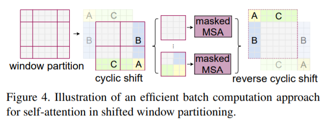
Layer l+1에서는 각 windows에 속한 patch 크기의 반으로 나누어 각 축을 $\left(\frac{P}{2}, \frac{M}{2}, \frac{M}{2}\right)=(2,2,2)$ 이동시킵니다. 따라서 Layer l+1은 3 x 3 x 3 =27개의 windows로 구성되게 됩니다. windows의 갯수는 늘어났지만 efficient batch computation을 위한 masking mechanism으로 인해 연산량은 Layer 1과 같은 2 x 2 x 2의 8로 유지하게 됩니다.
- Swin transformer(Efficient batch computation for shifted configuration)
- mmaction/models/backbones/swin_transformer.py
def window_partition(x, window_size):
    """
    Args:
        x: (B, D, H, W, C)
        window_size (tuple[int]): window size

    Returns:
        windows: (B*num_windows, window_size*window_size, C)
    """
    B, D, H, W, C = x.shape
    x = x.view(B, D // window_size[0], window_size[0], H // window_size[1], window_size[1], W // window_size[2], window_size[2], C)
    windows = x.permute(0, 1, 3, 5, 2, 4, 6, 7).contiguous().view(-1, reduce(mul, window_size), C)
    return windows

def get_window_size(x_size, window_size, shift_size=None):
    use_window_size = list(window_size)
    if shift_size is not None:
        use_shift_size = list(shift_size)
    for i in range(len(x_size)):
        if x_size[i] <= window_size[i]:
            use_window_size[i] = x_size[i]
            if shift_size is not None:
                use_shift_size[i] = 0

    if shift_size is None:
        return tuple(use_window_size)
    else:
        return tuple(use_window_size), tuple(use_shift_size)
3D Relative Position Bias
Transformer아키텍쳐는 image를 patch단위로 나누어 sequencial하게 구성되는 만큼 각 patch의 position 정보가 필요합니다. 종래의 방법에서는 Sinusoids 함수를 이용한 absolute positional encoding 방식을 사용해 왔지만 최근에는 다양한 position embedding 연구들이 나오고 있고 본 논문에서는 Relative Postional encoding을 사용하였습니다. 3D relative position bias는 $B \in \mathbb{R}^{P^{2} \times M^{2} \times M^{2}}$에 각각의 head는 $\text { Attention }(Q, K, V)=\operatorname{SoftMax}\left(Q K^{T} / \sqrt{d}+B\right) V$로 정의가 되고 $Q, K, V \in \mathbb{R}^{P M^{2} \times d}$ 각 3D window의 토큰과 dimension의 곱으로 나타낼 수 있습니다. relative position의 axis는 시간축 [−P + 1, P − 1]와 공간축 [−M + 1, M − 1]에 속하게 됩니다. 따라서 파라미터를 더 작은 영역 $\hat{B} \in \mathbb{R}^{(2 P-1) \times(2 M-1) \times(2 M-1)}$의 범위의 $\hat{B}$로 정의할 수 있습니다.
- mmaction/models/backbones/swin_transformer.py
# define a parameter table of relative position bias
        self.relative_position_bias_table = nn.Parameter(
            torch.zeros((2 * window_size[0] - 1) * (2 * window_size[1] - 1) * (2 * window_size[2] - 1), num_heads))  # 2*Wd-1 * 2*Wh-1 * 2*Ww-1, nH

# get pair-wise relative position index for each token inside the window
        coords_d = torch.arange(self.window_size[0])
        coords_h = torch.arange(self.window_size[1])
        coords_w = torch.arange(self.window_size[2])
        coords = torch.stack(torch.meshgrid(coords_d, coords_h, coords_w))  # 3, Wd, Wh, Ww
        coords_flatten = torch.flatten(coords, 1)  # 3, Wd*Wh*Ww
        relative_coords = coords_flatten[:, :, None] - coords_flatten[:, None, :]  # 3, Wd*Wh*Ww, Wd*Wh*Ww
        relative_coords = relative_coords.permute(1, 2, 0).contiguous()  # Wd*Wh*Ww, Wd*Wh*Ww, 3
        relative_coords[:, :, 0] += self.window_size[0] - 1  # shift to start from 0
        relative_coords[:, :, 1] += self.window_size[1] - 1
        relative_coords[:, :, 2] += self.window_size[2] - 1

        relative_coords[:, :, 0] *= (2 * self.window_size[1] - 1) * (2 * self.window_size[2] - 1)
        relative_coords[:, :, 1] *= (2 * self.window_size[2] - 1)
        relative_position_index = relative_coords.sum(-1)  # Wd*Wh*Ww, Wd*Wh*Ww
        self.register_buffer("relative_position_index", relative_position_index)
3.3 Architecture Variants
논문에서는 4가지 타입의 Video Swin Transformer버전을 소개하였습니다. 기본적으로 windows size는 8 x 7 x 7로 설정하였고 각 query의 head dimension은 32로 MLP의 hidden dimension은 4x로 구성하였습니다.
• Swin-T: C = 96, layer numbers = {2, 2, 6, 2}, Model size 0.25x • Swin-S: C = 96, layer numbers ={2, 2, 18, 2}, Model size 0.5x • Swin-B: C = 128, layer numbers ={2, 2, 18, 2}, Model size 1x • Swin-L: C = 192, layer numbers ={2, 2, 18, 2}, Model size 2x
- configs/base/models/swin/swin_tiny.py
backbone=dict(
        type='SwinTransformer3D',
        patch_size=(4,4,4),
        embed_dim=96,
        depths=[2, 2, 6, 2],
        num_heads=[3, 6, 12, 24],
        window_size=(8,7,7),
        mlp_ratio=4.,
        qkv_bias=True,
        qk_scale=None,
        drop_rate=0.,
        attn_drop_rate=0.,
        drop_path_rate=0.2,
        patch_norm=True),
3.4 Initialization from Pre-trained Model
Swin Transformer에서 시간축이 추가된 Video Swin Transformer 구조로 first stage에서의 linear embedding layer와 relative position bias를 다르게 구성하였고 temporal dimension에 대해 유지하면서 채널의 크기는 2배씩 증가시켰습니다.
4 Experiments
4.1 Setup
Datasets
평가 데이터 셋은 3가지가 사용되었는데 각 dataset에 대한 top-1과 top-5 정확도를 기록하였습니다. ~240k의 training video와 20k의 validation video로 400개의 human action category로 구성되어 있는 Kinetics-400(K400)과 K400에서 확장된 600개의 human action category를 ~370k의 training video와 28.3k의 validation video로 구성된 Kinetics-600(K600)과 temporal modeling을 위한 ~168.9k의 training video와 24.7k의 validation으로 174개의 class로 구성된 Something-Something V2 (SSv2)를 사용하였습니다.
Implementation Details
Video Swin Transformer는 OpenMMLab의 mmaction2를 기반으로 구현되어 있습니다. 또한 각 데이터셋 별로 config_file.py(e.g. configs/recognition/swin/swin_tiny_patch244_window877_kinetics400_1k.py)을 별도로 만들어 튜닝 및 평가가 가능합니다.
- configs/recognition/swin/swin_base_patch244_window877_kinetics400_1k.py
train_pipeline = [
    dict(type='DecordInit'),
    dict(type='SampleFrames', clip_len=32, frame_interval=2, num_clips=1),
    dict(type='DecordDecode'),
    dict(type='Resize', scale=(-1, 256)),
    dict(type='RandomResizedCrop'),
    dict(type='Resize', scale=(224, 224), keep_ratio=False),
    dict(type='Flip', flip_ratio=0.5),
    dict(type='Normalize', **img_norm_cfg),
    dict(type='FormatShape', input_format='NCTHW'),
    dict(type='Collect', keys=['imgs', 'label'], meta_keys=[]),
    dict(type='ToTensor', keys=['imgs', 'label'])
]
val_pipeline = [
    dict(type='DecordInit'),
    dict(
        type='SampleFrames',
        clip_len=32,
        frame_interval=2,
        num_clips=1,
        test_mode=True),
    dict(type='DecordDecode'),
    dict(type='Resize', scale=(-1, 256)),
    dict(type='CenterCrop', crop_size=224),
    dict(type='Flip', flip_ratio=0),
    dict(type='Normalize', **img_norm_cfg),
    dict(type='FormatShape', input_format='NCTHW'),
    dict(type='Collect', keys=['imgs', 'label'], meta_keys=[]),
    dict(type='ToTensor', keys=['imgs'])
]
evaluation = dict(
    interval=5, metrics=['top_k_accuracy', 'mean_class_accuracy'])
optimizer = dict(type='AdamW', lr=1e-3, betas=(0.9, 0.999), weight_decay=0.05,
                 paramwise_cfg=dict(custom_keys={'absolute_pos_embed': dict(decay_mult=0.),
                                                 'relative_position_bias_table': dict(decay_mult=0.),
                                                 'norm': dict(decay_mult=0.),
                                                 'backbone': dict(lr_mult=0.1)}))
lr_config = dict(
    policy='CosineAnnealing',
    min_lr=0,
    warmup='linear',
    warmup_by_epoch=True,
    warmup_iters=2.5
)
4.2 Comparison to state-of-the-art
Something-Something v2
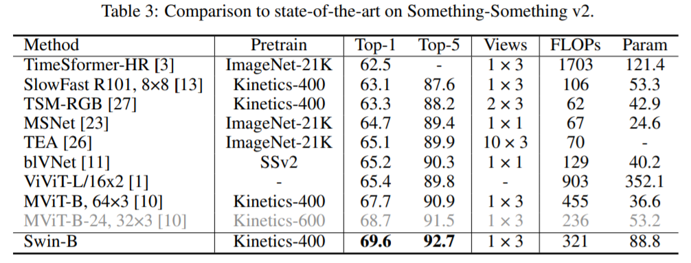
SSv2에서 최고 성능을 보여주었던 MViT-B-24보다 Swin-B가 더 나은 성능을 보여주고 있습니다. 또한 Swin-L과 같은 큰 모델을 사용하고 input resolution을 384 x 384로 크게 하면 성능을 더 개선할 수 도 있습니다.
- configs/recognition/swin/swin_base_patch244_window1677_sthv2.py
train_pipeline = [
    dict(type='DecordInit'),
    dict(type='SampleFrames', clip_len=32, frame_interval=2, num_clips=1, frame_uniform=True),
    dict(type='DecordDecode'),
    dict(type='Resize', scale=(-1, 256)),
    dict(type='RandomResizedCrop'),
    dict(type='Resize', scale=(224, 224), keep_ratio=False),
    dict(type='Flip', flip_ratio=0),
    dict(type='Imgaug', transforms=[dict(type='RandAugment', n=4, m=7)]),
    dict(type='Normalize', **img_norm_cfg),
    dict(type='RandomErasing', probability=0.25),
    dict(type='FormatShape', input_format='NCTHW'),
    dict(type='Collect', keys=['imgs', 'label'], meta_keys=[]),
    dict(type='ToTensor', keys=['imgs', 'label'])
]
val_pipeline = [
    dict(type='DecordInit'),
    dict(
        type='SampleFrames',
        clip_len=32,
        frame_interval=2,
        num_clips=1,
        frame_uniform=True,
        test_mode=True),
    dict(type='DecordDecode'),
    dict(type='Resize', scale=(-1, 256)),
    dict(type='CenterCrop', crop_size=224),
    dict(type='Flip', flip_ratio=0),
    dict(type='Normalize', **img_norm_cfg),
    dict(type='FormatShape', input_format='NCTHW'),
    dict(type='Collect', keys=['imgs', 'label'], meta_keys=[]),
    dict(type='ToTensor', keys=['imgs'])
]
model=dict(backbone=dict(patch_size=(2,4,4), window_size=(16,7,7), drop_path_rate=0.4),
           cls_head=dict(num_classes=174),
           test_cfg=dict(max_testing_views=2),
           train_cfg=dict(blending=dict(type='LabelSmoothing', num_classes=174, smoothing=0.1)))
4.3 Ablation Study
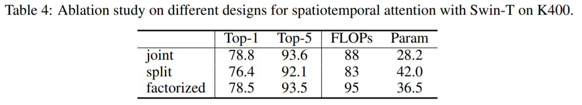
Different designs for spatiotemporal attention
spatiotemporal attention을 적용하기 위한 3가지 design으로 joint, split and factorized로 설계하였고 Spatial과 Temporal attention을 별도로 보는 split나 factorized보다 동일 attention layer에서 수행하는 joint version이 가장 좋은 성능을 보여주고 있습니다.
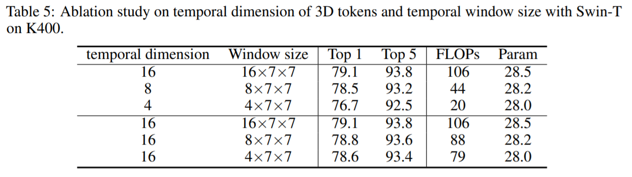
Temporal dimension of 3D tokens and Temporal window size
3D Token이 긴 시간축으로 보게될 경우 정확도는 올라가지만 높은 연산량과 느린 처리 속도의 한계가 있습니다. Temporal Windows size의 경우에도 같은 결과를 보이고 있습니다.
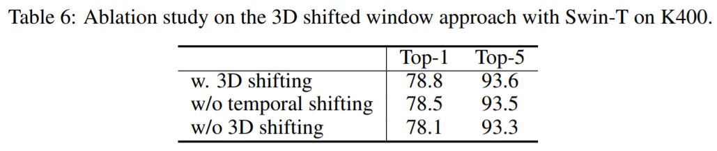
3D shifted windows
3D shifted windows의 유무와 temporal의 shifting에 따라 성능의 차이가 나타납니다.
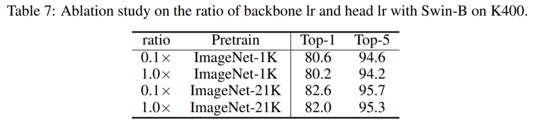
Ratio of backbone/head learning rate
ImageNet으로 Pretrin된 모델의 learning rate에 따라 성능의 차이가 나고 낮은 learning rate값이 더 좋은 성능을 보여주고 있습니다. K400의 데이터로 fitting되는 과정에서 일반화를 위해서 참고해야 할 사항인 것 같습니다.
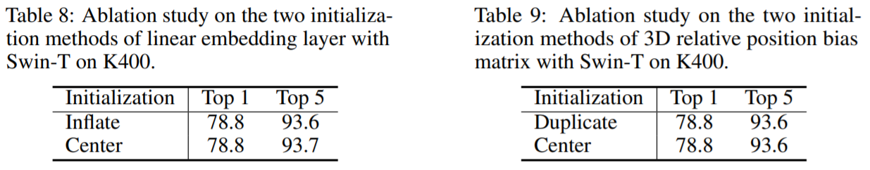
Initialization on linear embedding layer and 3D relative position bias matrix
ViViT[2]에서 소개된 linear embedding layer에 Cetner initialization(Center Frame를 제외하고 0으로 설정)과 Inflate initialization(전체 Frame의 Embedding을 시간축으로 나누어 평균으로 설정)의 경우 성능 차이가 거의 없었고 relative position bias의 경우에도 Duplicate와 Center의 경우에도 차이가 없었습니다. (Default는 Inflate와 Duplicate로 설정)
5 Conclusion
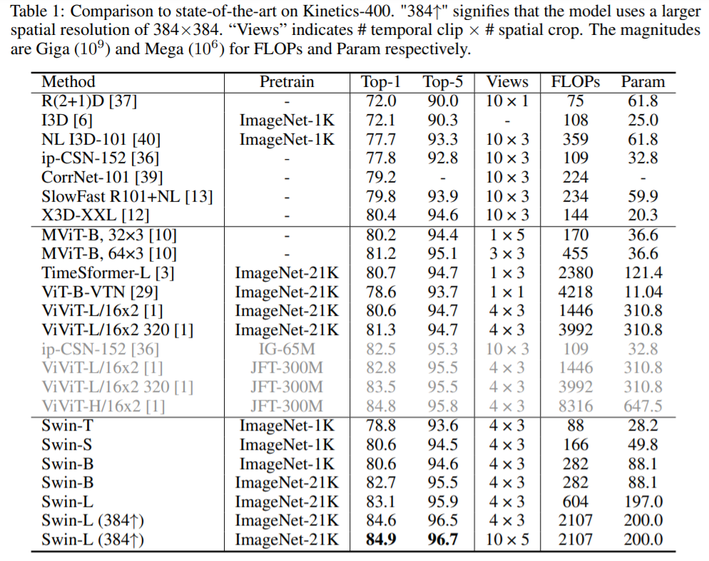
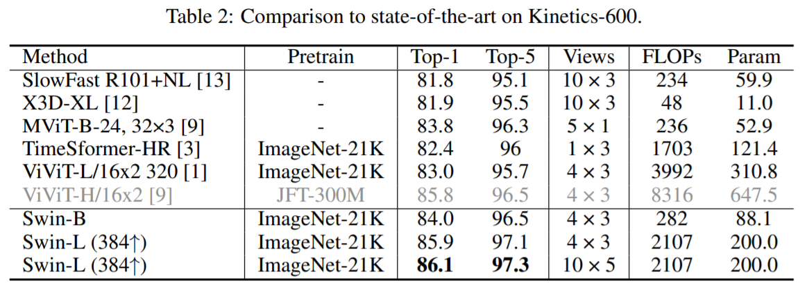
2D 정보상의 image recognition에서 Swin Transformer적용을 통해 SOTA를 달성하고 temporal축이 확장된 Video Swin Transformer를 통해서도 가장 많은 평가 데이터셋으로 활용되는 Kinetics-400, Kinetics-600, Something-Something v2에서도 SOTA를 달성하였습니다.
6 Reference
[1] Liu, Ze et al. “Swin Transformer: Hierarchical Vision Transformer using Shifted Windows.” arXiv, 2021
[2] A. Arnab et al., “ViViT: A Video Vision Transformer,” arXiv, 2021.
Reviewed by Susang Kim