Improved Multiscale Vision Transformers for Classification and Detection
2021년 12월 2일 arXiv에 올라온 Facebook의 MViT Version 2인 Improved Multiscale Vision Transformers for Classification and Detection을 Review하고자 합니다.
Abstract
Multiscale Vision Transformers (MViT)는 image와 video classification 및 object detection에서 최고의 성능을 보여왔고 본 논문에서 소개하는 MViT-v2에서는 decomposed relative positional embeddings과 residual pooling connections을 도입하여 정확도와 연산량에서 더 나은 성능을 확보하였을 뿐만 아니라 Visual Recognition에서 가장 많이 평가되는 3가지 도메인에서 SOTA를 달성하였습니다.(MViT has state-of-the-art performance : 88.8% accuracy on ImageNet classification, 56.1 APbox on COCO object detection, 86.1% on Kinetics-400 video classification.)
1 Introduction
Visual recognition을 위한 아키텍쳐는 CNN기반 아키텍쳐에서 최근 Vision Transformer 아키텍쳐의 등장에 따라 다양한 도메인에서 연구가 진행되어 되어 왔습니다. Vision Transformer의 경우 Transformer내의 Self-Attention block에서 scale에 따라 연산량과 메모리가 quadratic하게 증가하는 특징이 있습니다. 이를 해결하기 위해 최신 Transformer 아키텍쳐인 Swin Transformer에서는 local window attention을 적용하였고 MViT에서는 pooling attention을 적용하여 개선할 수 있었습니다.
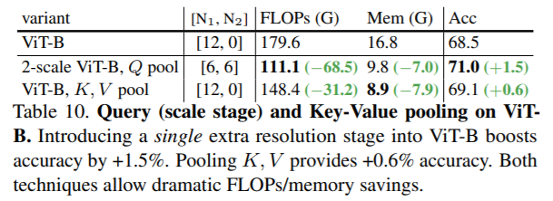
[Table - MViT-v1 논문에서 ViT를 2개의 Stage로 나누어 Pooling을 적용했을때의 성능 비교]
MViT-v1에 적용된 Pooling Attention에 따라 FLOPs는 감소하고 Acc는 향상된 것을 확인할 수 있습니다.
2. Related Work
Computer vision에서 지금껏 CNN이 backbone으로 많이 활용되어 왔습니다. Vision transformers의 경우 ViT의 등장 이후 발전되어 오면서 CNN의 성능을 능가하게 되었고 본 논문에서도 MViT-v2를 통해 Classification뿐만 아니라 Detection, Video recognition에서도 기존의 방법들보다 더 나은 성능을 보여주고 있습니다.
3. Revisiting Multiscale Vision Transformers
MViT-v1은 각 stage별로 resolution을 줄이고 channel을 확대하는 방법으로 각 Stage에 Pooling Attention이 적용되어 있습니다. input sequence인 $X ∈ R^{L×D}$에서 $W_Q, W_K, W_V ∈ R^{D×D}$을 통한 linear projection 후에 pooling operator $(P)$를 통해 아래와 같이 수식이 적용됩니다.
\[Q = P_Q (XW_Q), K = P_K(XW_K), V = P_V(XW_V )\]$P_Q(XW_Q)$을 통해 Pooling을 거친 output length는 $\widetilde{L}$은 $Q ∈ R^{\widetilde{L}×D}$ 로 줄어들게 됩니다. 그리고 Self Attention 연산을 거쳐 MViT-v1에서는 아래의 수식으로 적용이 되게됩니다.
\[Z := Attn (Q, K, V )=Softmax\left ( QK^T/\sqrt{d} \right)V,\]4. Improved Multiscale Vision Transformers
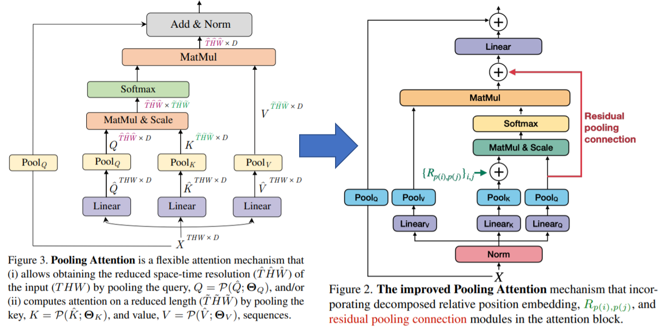
[그림 MViT-v1과 MViT-v2의 아키텍쳐 비교]
4.1. Improved Pooling Attention
Decomposed relative position embedding.
MViT-v1에서는 전체적인 구조보다는 Content 을 고려하여 token간의 연산에 중점을 두었고 permuation-invariant한 self-attention을 permutation-variant하기 위해 ViT에서 적용되었던 absolute positional encoding을 적용 하였습니다. absolute position의 경우 절대적인 위치 값으로 계산되기에 Vision이 가지고 있는 shift-invariance의 특징을 무시하기 마련입니다. (shift invariance는 translation invariance라고도 할 수 있는데 위치가 변하더라도 출력 값이 변하지 않는 다는 것을 의미하는데 이미지 내 patch의 위치가 같이 이동된다 하더라도 결과 값은 항상 같게 나온다는 의미입니다.)
MViT-v1에서 Multi Head Pooling Attention (MHPA) operator 모듈내의 patch간의 연산에서 pooling attention operation 적용을 통해 각 Stage별로 resolution이 감소하게 되고 (e.g. Pooling the query vector $P(Q; k; p; s)$, k : kernel, s : stride, p : padding)이 과정에서 input tensor length 값이 $\widetilde{L}= [\frac{L+2p-k}{s}]+1$로 줄어 들게 됩니다. 또한 pooling attention operation이 적용되면 상대적인 위치가 변하지 않더라도 absolute position 값이 바뀌게 됩니다. 이를 해결하기 위해 본 논문에서는 pooled self-attention 연산을 하는 과정에서 input patch사이에 pair-wise relationship을 고려하여 상대적인 위치를 연산하는 relative positional embedding을 적용하였습니다. 또한 Key Pooling 적용 이후에 relative position embedding(i.e. $R_{p(i),p(j)} ∈ R^d$) 을 적용하였고 이에따른 self-attention module은 아래와 같이 정의되게 됩니다.
$Attn(Q, K, V ) = Softmax\left ( (QK^T + E^{(rel)})/\sqrt{d} \right)V,$ where $E^{(rel)}{ ij} = Q_i· R{p(i),p(j)}$
MViT-v1에서의 관련 연구로 Positional Embedding에 따른 ablation study를 보면 space와 time를 분리한 경우에 Acc가 가장 높고 Param수도 상대적으로 적은 것을 확인할 수 있습니다.
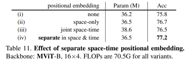
[Table - MViT-v1에서의 positional embedding관련한 ablation study]
본 논문에서도 $R_{p(i),p(j)}$의 연산량이 $O(TWH)$것을 줄이기 위해 각각을 height, width, temporal 축으로 나누어 $R_{p(i),p(j)} = R^h_{ h(i),h(j)} + R^w_{ w(i),w(j)} + R^t_{ t(i),t(j)}$로 계산을 하였고 연산량을 $O(T + W + H)$로 줄일 수 있었습니다. 특히 이는 초기 stage에서 resolution이 높은 경우 token의 수가 많기에 큰 효과가 있습니다.
Positional embeddings for video
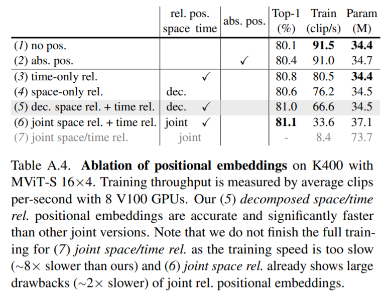
아래 table는 kinetics 400 dataset를 활용하여 decomposed relative positional embeddings관련한 ablation study를 나타내고 있고 decomposed의 경우에 성능도 좋고 학습속도가 빠른 것을 확인할 수 있습니다.
Residual pooling connection.
Attention block에서 pooling operator적용을 통해 메모리와 연산량을 감소시킬 수 있었습니다. $X ∈ R^{L×D}$에서 $W_Q, W_K, W_V ∈ R^{D×D}$을 linear projection 후 pooling operator을 통해 $Q = P_Q (XW_Q), K = P_K(XW_K), V = P_V(XW_V )$으로 연산이되어 input tensor length 값이 $\widetilde{L}= [\frac{L+2p-k}{s}]+1$로 줄어 들게 됩니다. 여기서 MViT-v1에서는 Key와 Value의 stride가 Query보다 커서 각 stage별로 pooling 시에 resolution만 downsampled되는 현상이 있었습니다. 따라서 Q tensor에 residual pooling connection을 두어 $Z := Attn (Q, K, V ) + Q$의 계산식과 같이 정보를 보존하면서도 연산량을 감소시킬 수 있게 되었습니다.
Residual pooling connection for detection and video.
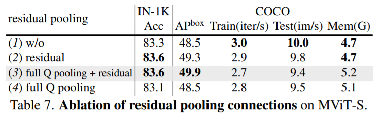
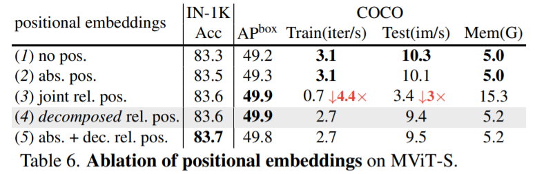
아래 table는 COCO dataset에 대한 residual pooling connections의 적용에 따른 Object Detection의 AP값을 확인할 수 있습니다.
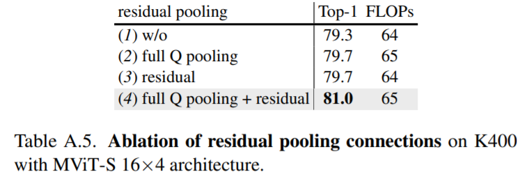
아래 table는 kinetics 400 dataset를 활용하여 residual pooling connections에 대한 정확도와 연산량을 확인할 수 있습니다.
4.2. MViT for Object Detection
MViT가 object detection과 instance segmentation에서 적용된 방법에 대해 설명하고자 합니다.
FPN integration.
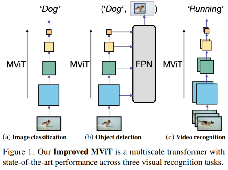
Hierarchical 구조인 MViT는 각 Stage별로 multiscale feature maps을 생성합니다. 따라서 Object Detection에서 Feature Pyramid Networks (FPN)와도 합칠 수 가 있습니다.
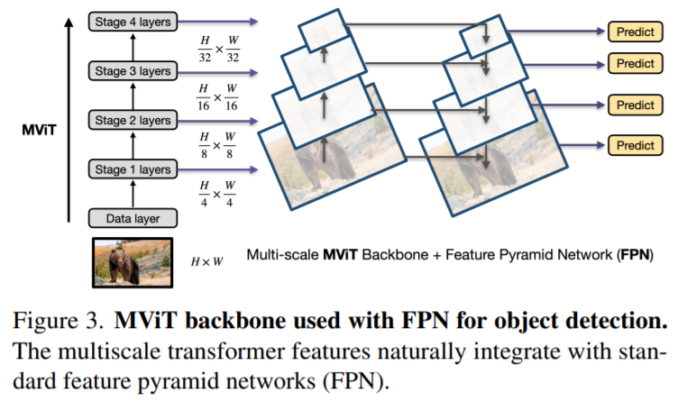
위 그림은 FPN과 MViT를 연결한 구조로 MASK R-CNN과 같은 다양한 Object Detection 아키텍쳐에 적용할 수 있습니다.
Hybrid window attention.
Self-attention은 토큰 수에 따라 quadratic한 연산량을 필요로 합니다. 따라서 High Resolution에서는 매우 큰 연산량이 필요로하기 마련인데 본 논문에서는 Hybrid형태인 Pooling Attention(마지막 3개의 Stage에 FPN적용)과 Swin Transformer에 적용된 Windows attention(i.e. windows별로 local self attention을 적용)을 통해 Hybrid window attention (Hwin)을 적용하였고 기존 Swin Transformer보다 더 나은 성능을 확인할 수 있었습니다.
Positional embeddings in detection.
Detection의 경우 Classification과는 다르게 resolution의 크기가 다양합니다. 따라서 처음 ImageNet pre-training weight로 초기화한 224 x 224 input 을 학습 시에 각각의 크기에 맞게 positional embedding를 적용하였습니다.
4.3. MViT for Video Recognition
MViT-v1에서는 Kinetics dataset을 활용한 scratch에 중점을 둔 반면 본 논문에서는 pre-training from ImageNet datasets을 활용한 실험을 진행하였습니다.
Initialization from pre-trained MViT
Video 영역에서의 MViT는 Image 영역과는 다른 점이 있습니다. 1) 2D patch가 아닌 space-time를 고려한 cube token인 3D로 token을 생성하였고 2) pooling operator의 경우에도 space-time를 고려한 feature map으로 처리하였습니다. 1),2)를 위해 center frame만 pre-trained weight를 사용하였고 다른 CNN Layer는 0으로 셋팅하였습니다. 3) relative positional embedding의 경우에도 space-time를 고려한 정보로 H+W+T로 decompose하여 처리하고 있습니다. (spatial의 경우 pre-trained weight를 사용하였고 temporal embedding는 0으로 셋팅하였습니다.)
4.4. MViT Architecture Variants
아래는 다양한 MViT아키텍쳐를 나타내고 있고 Tiny, Small, Base, Large, Huge의 5가지 종류에 대한 속성 값들을 나타내고 있습니다. (Key, Value의 첫번째 stage의 stride값은 4로 지정하였고 각 stage별로 resolution에 따라 적절히 줄이고 있습니다.)

5. Experiments: Image Recognition
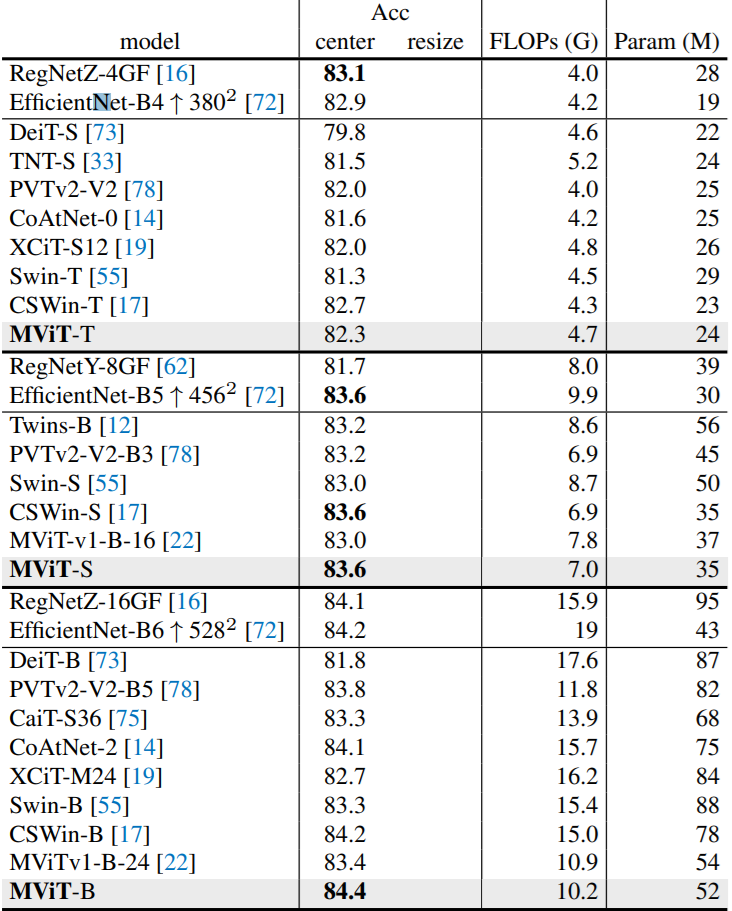
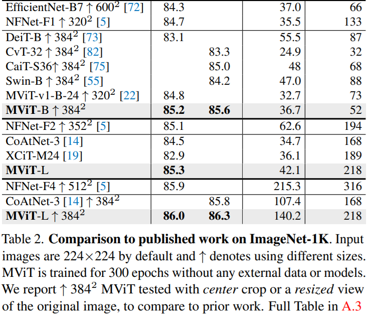
다양한 Resolution과 Data Scale에 따른 실험결과들입니다. 기존에 공개한 MViT-v1뿐만아니라 CNN이나 다른 Transformers 아키텍쳐(e.g. Swin Transformer, DeiT)보다 더 좋은 성능을 보여주는 것을 확인할 수 있습니다.
Results using ImageNet-1K.
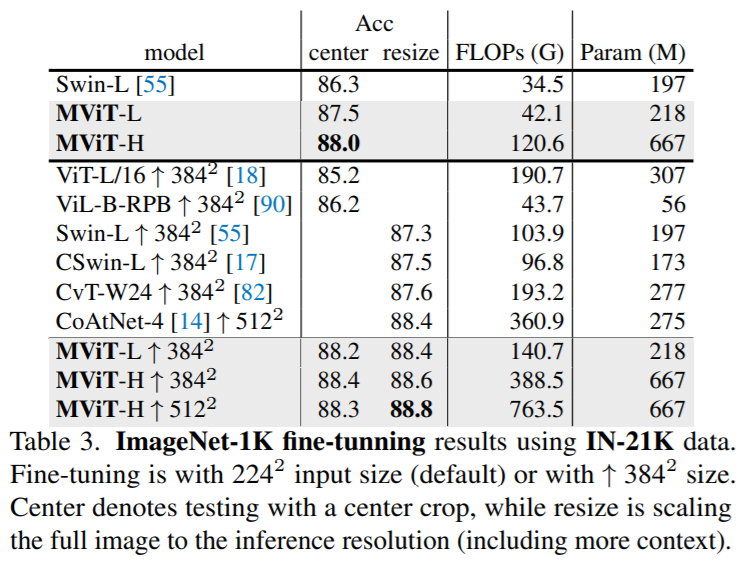
Results using ImageNet-21K.
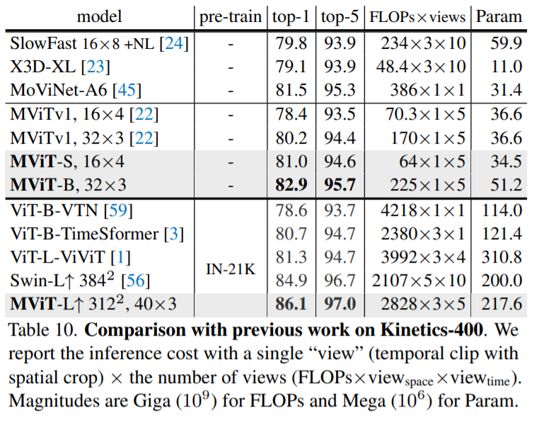
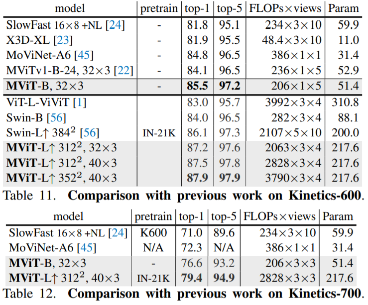
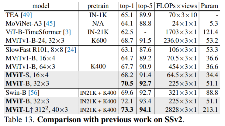
6. Experiments: Video Recognition
본 논문에서는 Kinetics-400(K400), Kinetics-600 (K600), Kinetics-700 (K700), Something-Something-v2 (SSv2) datasets으로 실험하였고 모든 dataset에서 SOTA를 달성하였습니다.
7. Conclusion
Visual recognition에 General hierarchical architecture 구조를 도입한 MViT는 다른 ViT 아키텍쳐 (e.g. Swin Transformer) 보다 더 나은 성능을 보여주었고 classification, object detection, instance segmentation, video recognition등 다양한 Task에서 SOTA를 달성하였습니다. Transformer기반 아키텍쳐는 현재 빠르게 발전되는 만큼 앞으로도 다양한 연구에 많이 활용될 것 같습니다.
Reference
[1] Fan, Haoqi et al. “Multiscale Vision Transformers.” ICCV, 2021.
[2] Liu, Ze et al. “Swin Transformer: Hierarchical Vision Transformer using Shifted Windows.” arXiv, 2021.
[3] P. Shaw et al. “Self-Attention with Relative Position Representations.” arXiv, 2018.
Reviewed by Susang Kim
-끝-